In today's data-driven landscape, ensuring the reliability and accuracy of your data warehouse is paramount. The cost of not testing your data can be astronomical, leading to critical business decisions based on faulty data and eroding trust. 

The path to rigorous data testing comes with its own set of challenges. In this article, I will highlight how you can confidently deploy your data pipelines by leveraging Starlake JSQLTranspiler and DuckDB, while also reducing costs. we will go beyond testing your transform usually written in SQL and see how we can also test our Ingestion jobs.

The art of mastering data pipelines​

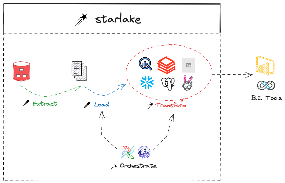
Mastering your data pipeline is a challenging art. A data pipeline generally contains the following phases:

• Collection: Extracting data from sources
• Ingestion: Loading the extracted data into the data warehouse
• Transformation: A phase that ultimately adds value to the collected data

The table below summarizes the tests run by Starlake on Load & Transform jobs:

Untested SQL costs​

Thanks to data pipelines unit testing, we drastically reduce the development cost. Not running tests seems to allow high project's velocity, thereby delivering value quickly. However, the cost of a feature does not stop at its simple development but encompasses all the efforts put in until the feature's completion. Below are some hidden costs.

• Identifying bugs
  • Without unit tests, verifying development requires deploying the project. This deployment raises challenging questions about the deployment strategy and its rollback or correction procedures.
  • Verification might be carried out by a separate QA team, sometimes even outside the project team. This can lead to the use of feature flags to avoid deploying to production, complicating the implementation. Additionally, waiting for feedback from the QA team introduces delays, increasing the cost of fixing any bugs that arise.
  • Depending on the deployment strategy, verification may also be incomplete due to a lack of control over the test data used.
• Maintenance and Evolution Complexity
  • Many of us have faced a massive query and struggled to make modifications without disrupting existing functionality, all while aiming for improvements like optimizing processing time. Rigorous unit tests can help with this. They allow us to enhance the expected outcomes in current datasets, create new ones, and compare the modified query results with these expectations. This significantly reduces the risk of regression.
• Decreased productivity
  • The absence of automated tests often means manually re-running parts or all of the system to ensure correct integration, which can lead to spending time fixing collateral bugs and thus reducing overall productivity. As the project advances, more components need verification, making the process even more time-consuming. This significantly diminishes the willingness to refactor or revise code.
• Promoting expertise
  • Without unit tests, teams often assign the same tasks to the same people, which hinders skill development and increases the risk of knowledge loss due to turnover.
• Customer dissatisfaction
  • A project with uncertain product output quality often leads to dissatisfaction, frustration, and a loss of trust in the individual, the team, or the product.

We are all aware of the hidden costs associated with the absence of tests; in my opinion, these are the most significant. Therefore, we will explore how to manage a data pipeline.

Writing unit test in Starlake​

Suppose we have the following transform.

We test it by creating the following hierarchy:

This is then how it is executed

Starlake unit tests benefits​

Running tests on a local DuckDB database instead of the target Data Warehouse has the following advantages:

• Fast Feedback: Local execution is significantly faster than using a remote database due to network latency. Additionally, the local environment might be better suited for handling small volumes of test data.
• No Execution Cost: Depending on the pricing model of the target database, creating temporary resources and executing queries can incur both execution and storage costs.
• Setup and Cleanup of Automated Tests: Guarantee of resource isolation.
• Credential Issues: Running tests against a target database requires credentials, which may pose security risks.

Conclusion​

In this article, we have demonstrated how adopting unit testing, a crucial practice for software engineers, can significantly enhance the quality of our data pipelines. This approach not only reduces overall costs in the medium to long term but also ensures the maintenance of dynamic and enduring documentation. Additionally, implementing unit tests is essential for rigorous CI/CD processes, enabling seamless continuous data pipeline deployment.

If you encounter any issues while performing your tests locally, please report them on the Starlake GitHub repository. Your feedback is invaluable in improving local test coverage, empowering more data engineers to deploy their work confidently and smoothly. For further discussions and support, join our team on Slack.

We greatly appreciate your contributions. If you found this article helpful, please star the project on GitHub and share it on your social networks to help us reach a broader audience.

Introduction​

Polars is often compared to Spark. In this post, I will highlight the main differences and the best use cases for each in my data engineering activities.

As a Data Engineer, I primarily focus on the following goals:

1. Parsing files, validating their input, and loading the data into the target data warehouse.
2. Once the data is loaded, applying transformations by joining and aggregating the data to build KPIs.

However, on a daily basis, I also need to develop on my laptop and test my work locally before delivering it to the CI pipeline and then to production.

What about my fellow data scientist colleagues? They need to run their workload on production data through their favorite notebook environment.

This post addresses the following points:

• How suitable each tool is for loading files into your data warehouse.
• How easy and powerful each tool is for performing transformations.
• How easy it is to test your code locally before deploying to the cloud

Load tasks​

Data loading seems easy at first glance, as almost all databases and APIs offer some sort of single-line command to load a few lines or millions of records quickly. However, this simplicity disappears when you encounter real-world cases such as:

• Fixed-width fields: These files are typically exported from mainframe databases.
• XML files: I sometimes work in the finance industry where SWIFT is a common XML file format that will be around for some time.
• Multi-character CSV: For example, where the separator consists of two characters like ||.
• File validation: You cannot trust the files you receive and need to check their content thoroughly.

Loading correct CSV or JSON files using Spark or Polars is straightforward. However, it is also straightforward using your favorite database command line utility, making this capabilities somewhat redundant and even slower than the native data warehouse load feature.

However, in real-world scenarios, you want to ensure the incoming file adheres to the expected schema and load a variety of file formats not supported natively. This is where Spark excels compared to Polars, as it allows for the parallel loading of your JSONL or CSV files and offers through map operations local and distributed validation of your incoming file.

As XML and multichar and multiline CSV are only supported by Spark, dealing with file parsing for data loading, Spark is definitely the most suitable solution.

Transform tasks​

Three interfaces are provided to transform data: SQL, Dafarames and Datasets.

SQL

SQL is the preferred language for most data analysts when it comes to computing aggregations. One of its key benefits is its widespread understanding, which eliminates the learning curve.

You can use SQL with both Spark and Polars, but Polars has significant limitations. It does not support SQL Window functions nor does it support the SQL statements for update, insert, delete, or merge operations.

Dataframes

Both Polars and Spark offer excellent support for DataFrames. The main added value of using DataFrames is the ability to reuse portions of code and access features not available in standard SQL, such as lambda functions, JSON handling and array manipulation.

Datasets

As a software engineer, I particularly appreciate Datasets. Datasets are typed DataFrames, meaning that syntax, column names, and types are checked at compile time. If you believe that statically typed languages greatly enhance code quality, then you understand the added value of datasets.

Datasets are only supported by Spark, allowing you to write clean, reusable, and statically typed transformations. They are available exclusively to statically typed languages such as Java or Scala.

Spark stands out as the only tool with complete support for SQL, DataFrames, and Datasets. Polars’ limited support for SQL makes it less suitable for my data engineering tasks.

Cloud Era​

At least 60% of the projects I have worked on are cloud-based, primarily targeting Amazon Redshift, Google BigQuery, Databricks, Snowflake, or Azure Synapse. All of these platforms offer serverless support for Spark, making it incredibly easy to run workloads by simply providing your PySpark script and letting the cloud provider handle the rest.

In the cloud environment, Spark is definitely the tool of choice as I see it.

Single node​

There has been much discussion about Spark being slow or too heavy for single-node computers. I was particularly interested in running this test since I currently execute most of my workloads on a single-node Google Cloud Run job with Spark embedded in my Docker image.

I decided to conduct this test on my almost 3-year-old MacBook Pro M1 Max with 64GB of memory. The test involved loading 27GB of CSV data, selecting a few attributes, computing metrics on those selected attributes, and then saving the results to a Parquet file.

I ran Spark with default settings and without any fine-tuning. This means it utilized all 10 cores of my MacBook Pro M1 Max but only 1 gigabyte of memory for execution.

::: note I could have optimized my Spark workload, but given the small size of the dataset (27GB of CSV), it didn't make sense. The default settings were sufficient. :::

Here are the results after a cold restart of my laptop before each test to ensure the test did not benefit from any operating system cache.

• Apache Spark pipeline took: 29 seconds

• Polars pipeline took: 56 seconds

::: note Rerunning Polars gave me 23 seconds instead of 56 seconds. This discrepancy is probably due to filesystem caching by the operating system. :::

Load and Save Test: Load a 27GB CSV file with 193 columns per record and save the result as parquet.

• Apache Spark pipeline took: 2mn 18s

• Polars pipeline took: 2mn 32s

Load parquet and filter on column value then return count : Load a 74 millions records parquet file with 193 columns, filter on 'model' column and return count.

• Apache Spark pipeline took: 3 seconds

• Polars pipeline took: 28 seconds

The table below summarises the results

Conclusion​

I don’t think it is time to switch from Spark to Polars, at least for those of us accustomed to the JVM, running workloads in the cloud, or even working on small datasets. However, Polars may be a perfect fit for those familiar with pandas.

As of today, Spark is the only framework I see that can handle both local and distributed workloads, adapt to on-premise and cloud serverless jobs, and provide the complete SQL support required for most of our transformations.

Introduction​

The advent of declarative programming through tools like Ansible and Terraform, has revolutionized infrastructure deployment by allowing developers to achieve intended goals without specifying the order of code execution.

This paradigm shift brings forth benefits such as reduced error rates, significantly shortened development cycles, enhanced code readability, and increased accessibility for developers of all levels.

This is the story of how a small team of developers crafted a platform that goes beyond the boundaries of conventional data engineering by applying a declarative approach to data extraction, loading, transformation and orchestration.

The Genesis​

Back in 2015, at the helm of ebiznext, a boutique data engineering company, we faced a daunting challenge. Our client, a prominent entity in need of a robust big data solution, sought to harness the power of Hadoop and Spark. Despite our modest size (20 people), we dared to compete against industry giants with tenfold resources (100.000+ headcount).

Our only chance to succeed was to innovate: we needed a data platform that could exponentially outperform the traditional ETL solutions pushed by our competitors. To build data pipelines these GUI based ETLs require an effort that is proportional to the number and complexity of the sources.

Determined to disrupt this norm, we embarked on a quest to devise a DevOps friendly platform capable of lightning-fast data ingestion from any source, without the drawbacks of ETLs or specialized engineering skills.

The day of the tender, our ability to deliver a solution that could load data in a few weeks instead of many months allowed us to stand out from the competition and win the project.

Expisode 1: Smartlake Emerges​

This left us with little choice but to embrace the declarative approach. Empowering business users, we devised a system where data formats and transformations could be described in simple JSON files. Smartlake wasn’t merely a code generator; it was a versatile engine, seamlessly ingesting diverse data formats, executing transformations, and orchestrating operations with unparalleled efficiency.

To streamline user interaction, we devised an intuitive Excel-to-JSON converter, enabling effortless specification of input formats. Thanks to Smartlake and its declarative approach, the business users were able to define load and transformation operations in a matter of minutes.

Smartlake Standout features

• Load almost any file format at Spark speed (CSV, JSON, XML, FIXED WITH, Multi-record types …) or Kafka topic

• Validate fields using user-defined schemas with user defined semantic types

• Apply transformations on the fly to data being loaded (GDPR, normalisation, computed fields ...) with and without schema evolution

• Sink to almost any target including Spark, Kafka, Elasticsearch.

Episode 2: Evolution to Starlake​

As the data landscape evolved, so did our vision. Cloud data warehouses emerged as formidable competitors to Spark for query execution. Recognizing this shift, we evolved Smartlake into Starlake, preserving its declarative essence while embracing YAML for enhanced readability. We maintained Spark’s prowess to run inside single or multiple container(s) for data ingestion, leveraging cloud data warehouses for query execution.

This strategic blend allowed us to optimize performance and cost-effectiveness based on specific workload requirements. The result was a reimagined platform, tailored for the cloud era, yet grounded in the principles of efficiency and simplicity that defined its inception.

The result is the Starlake OSS project that you can find on Github.

The capabilities of Starlake are extensively described here.

The people behind Starlake​

Smartlake, the precursor to Starlake, owes its existence to the collective efforts of numerous individuals, but a select few stand out for their exceptional contributions:

• Sam Bessalah With Sam’s presence, rallying others became effortless. His visionary outlook and knack for simplifying complexities proved transformative, setting a new standard for implementation.

• Olivier Girardot Every team has its coding wizard, and Olivier filled that role impeccably. From leveraging Spark codegen to exploring mathematical frameworks like matryoshka, he pushed the boundaries, mentoring the team with his expertise spanning Docker, Ansible, Python, Scala and Spark internals.

• Valentin Kasas Valentin championed functional programming in Scala. Introducing concepts like recursion schemes, he empowered the team to craft code that was not just functional but also elegant and maintainable.

As the journey progressed towards the cloud, long time data experts joined and made Starlake what it is today:

• Bounkong Khamphousone The speed and efficiency of Starlake’s extraction and load engines owe much to his contributions.

• Mohamad Kassir His direct involvement with customer projects and his in-depth knowledge of cloud platforms and business needs have been major assets in the evolution of Starlake.

• Abdelhamide EL ARIB An early contributor to the load engine, this foresight and execution prowess played a significant role in shaping the platform’s today capabilities.

• Stephane Manciot The developer behind Starlake’s declarative workflows on top of Airflow and Dagster, was pivotal in shaping its operational backbone.

• Cyrille Chépélov A master of codebase optimisation, Cyrille’s rewrite efforts were instrumental in ensuring the reentrant nature of Starlake’s API.

The next journey​

Today with hundreds of gigabytes of data loaded and transformed daily into thousands of tables in various data warehouses, we can confidently say that Starlake is battle tested and ready for the most demanding data engineering & analytics challenges.

As Starlake is, and will always be open source, join us in building a supportive community. Your insights and feature requests aren’t just welcome, they guide our roadmap.

Get Started with Starlake:

• Check-out the other features

• Explore our documentation

Join our community on GitHub

P.S. Please star the repository: https://github.com/starlake-ai/starlake. Also, any issue or enhancement with Starlake, please just report it. It will fall under the scope of gracious care taking of course.

Data exposition strategies​

Data may be exposed using views or authorized views and more recently using Row / Column level security.

Historically, to restrict access on specific columns or rows in BigQuery, one can create a (authorized) view with a SQL request like the one below:

BigQuery Views require to grant access for the end users to the table on top of which the view is created. To bypass that limitation, BigQuery provide Authorized views. However, Authorized views come with the following restrictions:

1. The underlying table is accessed through the authorized view where the end user is impersonated, loosing thus at the table level, the identity of the user making the request.

2. Each restriction policy require to define a specific authorized view making it difficult to identify who has access to what ?

3. Authorized views need to be updated whenever a schema evolution on the underlying table bring in a sensitive field that need to be excluded or a field that need to be included in the view. In the example below, the new column "description" need to be added to the authorized view if we want it .

That's where Row Level Security and Column Level security features natively supported by BigQuery come in.

BigQuery Row Level Security​

Row Level Security restrict access to the rows based on the conditions set in the where clause using the custom SQL statement below:

Big Query Column Level Security​

Column level security in BigQuery is managed using a taxonomy. This taxonomy is a hierarchy of policy tags describing the table attributes or other resources. By assigning access rights to a tag, we restrict access to any resource tagged using this specific tag and this applies to BigQuery table fields.

In our example, restricting access to specific user/group/sa to the column price require the following steps:

1. In Cloud Data Catalog/Policy Tags, create a Taxonomy. Note that Enfore access control should be checked.

2. Assign permissions for each policy tag you defined

3. Tag restricted columns in the BigQuery schema editor.

BigQuery RLS/CLS benefits​

Using BigQuery row and column level security features bring several benefits:

• There is no need to create extra views
• Users use the same name for the table but with different access rights
• A company-wide taxonomy is defined allowing better Data Management
• Access rights to a new column in the table are automatically handled

A word about RLS and CLS in Starlake​

Ingesting Data into BigQuery cannot be considered complete without taking into account the access level restrictions on the target table. Starlake will handle for you all the scripting required to secure BigQuery rows and columns using a YAML declarative syntax to make sure that your tables are secured in BigQuery:

  - name: "PRODUCT"
    rls:
      - name: "my-rls"
        predicate: "category like 'Food'"
        grants:
          - "user:me@company.com"
          - "group:financegroup@company.com"
          - "sa:serviceacount@gserviceaccount.com"
    attributes:
      - name: "id"
        accessPolicy: PII

Data Loading strategies​

When loading data into BigQuery, you may want to:

• Overwrite the existing data and replace it with the incoming data.
• Append incoming data to existing
• Dynamic partition Overwrite where only the partitions to which the incoming data belong to are overwritten.
• Merge incoming data with existing data by keeping the newest version of each record.

For performance reasons, when having huge amount of data, tables are usually split into multiple partitions. BigQuery supports range partitioning which are uncommon and date/time partitioning which is the most widely used type of partitioning. The diagram below shows our initial table partitioned by the date field.

Let's assume we receive the following data that we need to ingest into the table:

The strategies above will produce respectively the results below:

There is no good or bad strategy, the use of one of the strategies above depends on the use case. Some use case examples for each of the strategies are:

• Overwrite mode may be useful when you receive every day the list of all product names.
• Append mode may be useful when you receive daily sales.
• Dynamic Partition Overwrite mode may be useful when you ingested the first time a partition, and you need to ingest it again with a different set of data and thus alter only that partition.
• Merge mode may be useful when you receive product updates every day and that you need to keep only the last version of each product.

Spark How-to

Apache Spark SQL connector for Google BigQuery makes BigQuery a first class citizen as a source and sink for Spark jobs.

Append and Overwrite modes in Spark​

BigQuery is supported by Spark as a source and sink through the Spark BigQuery connector

Spark comes out of the box with the ability to append or overwrite existing data using a predefined save mode:

val incomingDF = ... // Incoming data loaded with the correct schema
val bqTable = "project-id.dataset.table"
val saveMode = SaveMode.Overwrite // or SaveMode.Append fot he appending data
incomingDF.write
    .mode(saveMode)
    .partitionBy("date")
    .format("com.google.cloud.spark.bigquery")
    .option("table", bqTable)
    .save()

Dynamic Partition Overwrite mode in Spark​

To activate dynamic partitioning, you need to set the configuration below before saving the data using the exact same code above:

spark.conf.set("spark.sql.sources.partitionOverwriteMode","DYNAMIC")

Unfortunately, the BigQuery Spark connector does not support this feature (at the time of writing). We need to manually delete the partitions we want to overwrite first and then append the incoming data.

Assuming the table is partitioned by the field date and the incoming data loaded in the incomingDF dataframe, the code below will remove existing partitions that need to be overwritten.

val incomingDF = ... // Incoming data loaded with the correct schema
incomingDF
  .select(date_format(col("date"), "yyyyMMdd").cast("string"))
  .distinct()
  .collect()
  .map(_.getString(0))
  .foreach { partition =>
    bigQueryClient.deleteTable(TableId.of(datasetName, s"$table\$$partition"));
  }

bq rm -t 'project-id.dataset.table$YYYYMMDD'

We now need to append the incomingDF to mimic the dynamic partition overwrite feature:

val incomingDF = ... // Incoming data loaded with the correct schema
val bqTable = "project-id.dataset.table"
val saveMode = SaveMode.Append
incomingDF.write
    .mode(saveMode)
    .partitionBy("date")
    .format("com.google.cloud.spark.bigquery")
    .option("table", bqTable)
    .save()

Dynamic Partition Merge in Spark​

When you need to keep the last version of the record for each product, both BigQuery and Databricks (the company behind Spark in case you lived on the moon the last ten years) support the merge SQL statement:

MERGE INTO target_table
USING incoming_table
ON target_table.product = incoming_table.product
    WHEN NOT MATCHED
		THEN INSERT *
	WHEN MATCHED AND incoming_table.date > target_table.date THEN
		UPDATE SET *
/*
    WHEN MATCHED AND incoming_table.timestamp <= target_table.timestamp THEN
		SKIP
*/

Unfortunately the MERGE statement is not supported by Apache Spark. It is only supported by Databricks, its commercial version.

To do a merge using the Spark BigQuery connector, we need to do it by following the steps below:

Step 1: Create a dataframe with all the rows

val allRowsDF =
    incomingDF
    .unionByName(existingDF)

Step 2: group by product and order each product occurrence by date descending

val orderingWindow =
    Window
      .partitionBy("product")
      .orderBy(col("date").desc, col("product")))

val orderedDF =
    allRowsDF
        .withColumn("rownum", row_number.over(orderingWindow))

In the step 2 above, each product is ordered by date with the most recent one first (descending order). We identify it by the rownum column.

Step 3: Keep the most recent product

val toKeepDF =
    orderedDF
        .where(col("rownum") === 1)
        .drop("rownum")

Step 4: Overwrite existing partitions with the data we want to keep

val bqTable = "project-id.dataset.table"
val saveMode = SaveMode.Overwrite
toKeepDF.write
    .mode(saveMode)
    .partitionBy("date")
    .format("com.google.cloud.spark.bigquery")
    .option("table", bqTable)
    .save()

Starlake How-to​

Starlake is a declarative Ingestion Framework based on YAML description files.
The 4 ingestion strategies described above are supported through the settings below:

     name: "mydb"
     directory: "..."
+    metadata:
    schemas:
      - name: "mytable"
        pattern: "data-.*.csv"
        metadata:
          writeStrategy:
            type: "OVERWRITE"
       attributes:
          - name: "date"
            type: "date"
            rename: "id"
          - name: "product"
            type: "string"
          - name: "price"
            type: "decimal"

     name: "mydb"
     directory: "..."
+    metadata:
    schemas:
      - name: "mytable"
        pattern: "data-.*.csv"
        metadata:
          writeStrategy:
            type: "APPEND"
        attributes:
          - name: "date"
            type: "date"
            rename: "id"
          - name: "product"
            type: "string"
          - name: "price"
            type: "decimal"

    name: "mydb"
    directory: "..."
+   metadata:
    schemas:
      - name: "mytable"
        pattern: "data-.*.csv"
        metadata:
          strategy:
            type: "OVERWRITE_BY_PARTITION"
          sink:
            partition:
              - "date"
       attributes:
          - name: "date"
            type: "date"
            rename: "id"
          - name: "product"
            type: "string"
          - name: "price"
            type: "decimal"

     name: "mydb"
     directory: "..."
+    metadata:
    schemas:
      - name: "mytable"
        pattern: "data-.*.csv"
        metadata:
          strategy:
            type: "OVERWRITE_BY_KEY_AND_TIMESTAMP"
            key: ["product"]
            timestamp: "date"
        attributes:
          - name: "date"
            type: "date"
          - name: "product"
            type: "string"
          - name: "price"
            type: "decimal"

Pipelining fast data is big. Pipelining big data fast is bigger. :)