3 posts tagged with "Spark"

View All Tags

Polars versus Spark

· 6 min read
Hayssam Saleh
Starlake Core Team

Introduction

Polars is often compared to Spark. In this post, I will highlight the main differences and the best use cases for each in my data engineering activities.

As a Data Engineer, I primarily focus on the following goals:

  1. Parsing files, validating their input, and loading the data into the target data warehouse.
  2. Once the data is loaded, applying transformations by joining and aggregating the data to build KPIs.

However, on a daily basis, I also need to develop on my laptop and test my work locally before delivering it to the CI pipeline and then to production.

What about my fellow data scientist colleagues? They need to run their workload on production data through their favorite notebook environment.

This post addresses the following points:

  • How suitable each tool is for loading files into your data warehouse.
  • How easy and powerful each tool is for performing transformations.
  • How easy it is to test your code locally before deploying to the cloud

Load tasks

Data loading seems easy at first glance, as almost all databases and APIs offer some sort of single-line command to load a few lines or millions of records quickly. However, this simplicity disappears when you encounter real-world cases such as:

  • Fixed-width fields: These files are typically exported from mainframe databases.
  • XML files: I sometimes work in the finance industry where SWIFT is a common XML file format that will be around for some time.
  • Multi-character CSV: For example, where the separator consists of two characters like ||.
  • File validation: You cannot trust the files you receive and need to check their content thoroughly.

Loading correct CSV or JSON files using Spark or Polars is straightforward. However, it is also straightforward using your favorite database command line utility, making this capabilities somewhat redundant and even slower than the native data warehouse load feature.

However, in real-world scenarios, you want to ensure the incoming file adheres to the expected schema and load a variety of file formats not supported natively. This is where Spark excels compared to Polars, as it allows for the parallel loading of your JSONL or CSV files and offers through map operations local and distributed validation of your incoming file.

As XML and multichar and multiline CSV are only supported by Spark, dealing with file parsing for data loading, Spark is definitely the most suitable solution.

Transform tasks

Three interfaces are provided to transform data: SQL, Dafarames and Datasets.

SQL

SQL is the preferred language for most data analysts when it comes to computing aggregations. One of its key benefits is its widespread understanding, which eliminates the learning curve.

You can use SQL with both Spark and Polars, but Polars has significant limitations. It does not support SQL Window functions nor does it support the SQL statements for update, insert, delete, or merge operations.

Dataframes

Both Polars and Spark offer excellent support for DataFrames. The main added value of using DataFrames is the ability to reuse portions of code and access features not available in standard SQL, such as lambda functions, JSON handling and array manipulation.

Datasets

As a software engineer, I particularly appreciate Datasets. Datasets are typed DataFrames, meaning that syntax, column names, and types are checked at compile time. If you believe that statically typed languages greatly enhance code quality, then you understand the added value of datasets.

Datasets are only supported by Spark, allowing you to write clean, reusable, and statically typed transformations. They are available exclusively to statically typed languages such as Java or Scala.

Spark stands out as the only tool with complete support for SQL, DataFrames, and Datasets. Polars’ limited support for SQL makes it less suitable for my data engineering tasks.

Cloud Era

At least 60% of the projects I have worked on are cloud-based, primarily targeting Amazon Redshift, Google BigQuery, Databricks, Snowflake, or Azure Synapse. All of these platforms offer serverless support for Spark, making it incredibly easy to run workloads by simply providing your PySpark script and letting the cloud provider handle the rest.

In the cloud environment, Spark is definitely the tool of choice as I see it.

Single node

There has been much discussion about Spark being slow or too heavy for single-node computers. I was particularly interested in running this test since I currently execute most of my workloads on a single-node Google Cloud Run job with Spark embedded in my Docker image.

I decided to conduct this test on my almost 3-year-old MacBook Pro M1 Max with 64GB of memory. The test involved loading 27GB of CSV data, selecting a few attributes, computing metrics on those selected attributes, and then saving the results to a Parquet file.

I ran Spark with default settings and without any fine-tuning. This means it utilized all 10 cores of my MacBook Pro M1 Max but only 1 gigabyte of memory for execution.

::: note I could have optimized my Spark workload, but given the small size of the dataset (27GB of CSV), it didn't make sense. The default settings were sufficient. :::

Here are the results after a cold restart of my laptop before each test to ensure the test did not benefit from any operating system cache.

  • Apache Spark pipeline took: 29 seconds

  • Polars pipeline took: 56 seconds

::: note Rerunning Polars gave me 23 seconds instead of 56 seconds. This discrepancy is probably due to filesystem caching by the operating system. :::

Load and Save Test: Load a 27GB CSV file with 193 columns per record and save the result as parquet.

  • Apache Spark pipeline took: 2mn 18s

  • Polars pipeline took: 2mn 32s

Load parquet and filter on column value then return count : Load a 74 millions records parquet file with 193 columns, filter on 'model' column and return count.

  • Apache Spark pipeline took: 3 seconds

  • Polars pipeline took: 28 seconds

The table below summarises the results

TaskSpark 1GB memoryPolars All the available memory
Load CSV, aggregate and save the aggregation as parquet29s56s
Load CSV and Save parquet2mn 18s2mn 32s
Load Parquet, filter and count3s28s

Conclusion

I don’t think it is time to switch from Spark to Polars, at least for those of us accustomed to the JVM, running workloads in the cloud, or even working on small datasets. However, Polars may be a perfect fit for those familiar with pandas.

As of today, Spark is the only framework I see that can handle both local and distributed workloads, adapt to on-premise and cloud serverless jobs, and provide the complete SQL support required for most of our transformations.

Column and Row Level Security in BigQuery

· 3 min read
Hayssam Saleh
Starlake Core Team Member

Data exposition strategies

Data may be exposed using views or authorized views and more recently using Row / Column level security.

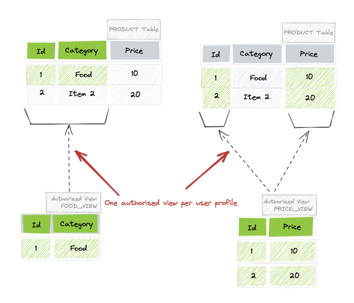
Historically, to restrict access on specific columns or rows in BigQuery, one can create a (authorized) view with a SQL request like the one below:

CLS / RLS using Views

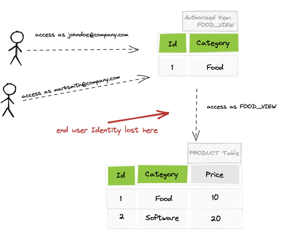
BigQuery Views require to grant access for the end users to the table on top of which the view is created. To bypass that limitation, BigQuery provide Authorized views. However, Authorized views come with the following restrictions:

  1. The underlying table is accessed through the authorized view where the end user is impersonated, loosing thus at the table level, the identity of the user making the request. Impersonation

  2. Each restriction policy require to define a specific authorized view making it difficult to identify who has access to what ? Multiplication of Authorized Views

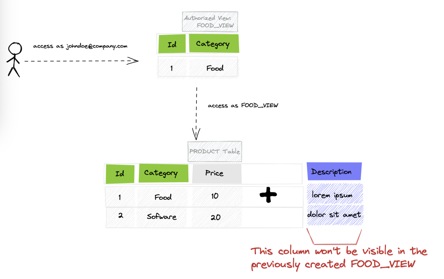
  3. Authorized views need to be updated whenever a schema evolution on the underlying table bring in a sensitive field that need to be excluded or a field that need to be included in the view. In the example below, the new column "description" need to be added to the authorized view if we want it . Multiplication of Authorized Views

That's where Row Level Security and Column Level security features natively supported by BigQuery come in.

BigQuery Row Level Security

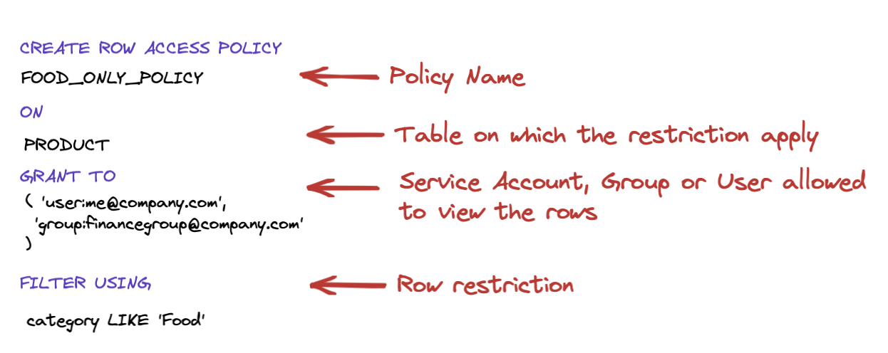
Row Level Security restrict access to the rows based on the conditions set in the where clause using the custom SQL statement below:

RLS

Big Query Column Level Security

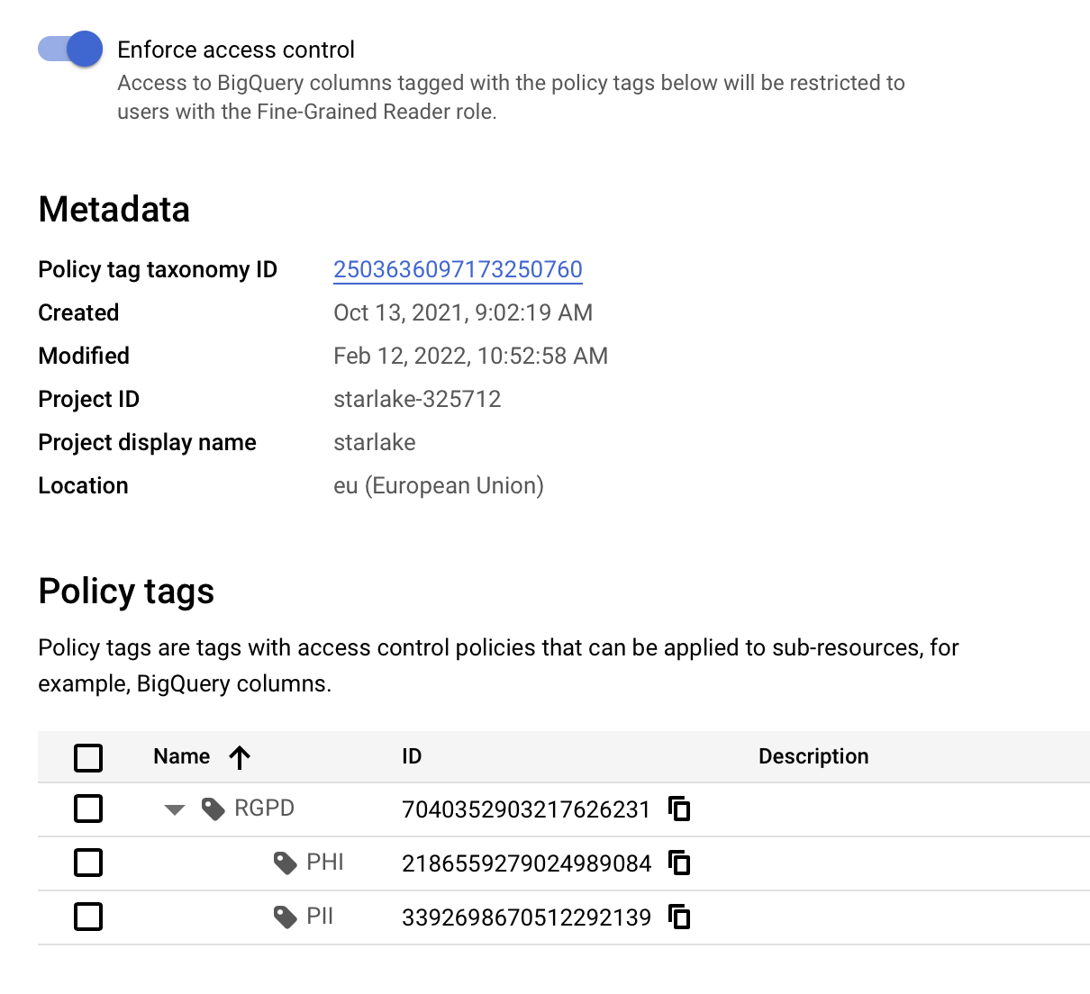
Column level security in BigQuery is managed using a taxonomy. This taxonomy is a hierarchy of policy tags describing the table attributes or other resources. By assigning access rights to a tag, we restrict access to any resource tagged using this specific tag and this applies to BigQuery table fields.

In our example, restricting access to specific user/group/sa to the column price require the following steps:

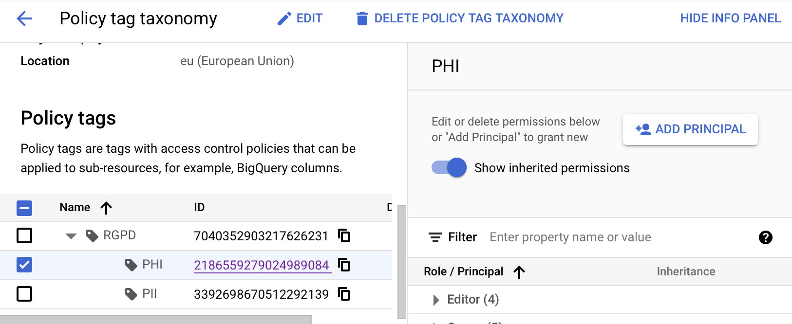
  1. In Cloud Data Catalog/Policy Tags, create a Taxonomy. Note that Enfore access control should be checked.

CLS Taxonomy

  1. Assign permissions for each policy tag you defined

CLS Access

  1. Tag restricted columns in the BigQuery schema editor. CLS Assign
tip

Assigning policy tags may be done using the bq load/update command line tool

BigQuery RLS/CLS benefits

Using BigQuery row and column level security features bring several benefits:

  • There is no need to create extra views
  • Users use the same name for the table but with different access rights
  • A company-wide taxonomy is defined allowing better Data Management
  • Access rights to a new column in the table are automatically handled

A word about RLS and CLS in Starlake

Ingesting Data into BigQuery cannot be considered complete without taking into account the access level restrictions on the target table. Starlake will handle for you all the scripting required to secure BigQuery rows and columns using a YAML declarative syntax to make sure that your tables are secured in BigQuery:

Declarative Row Level & Column Level Security
  - name: "PRODUCT"
rls:
- name: "my-rls"
predicate: "category like 'Food'"
grants:
- "user:me@company.com"
- "group:financegroup@company.com"
- "sa:serviceacount@gserviceaccount.com"
attributes:
- name: "id"
accessPolicy: PII

Handling Dynamic Partitioning and Merge with Spark on BigQuery

· 7 min read
Hayssam Saleh
Starlake Core Team Member

Data Loading strategies

When loading data into BigQuery, you may want to:

  • Overwrite the existing data and replace it with the incoming data.
  • Append incoming data to existing
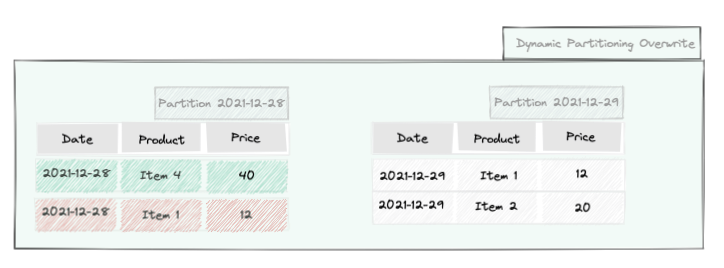
  • Dynamic partition Overwrite where only the partitions to which the incoming data belong to are overwritten.
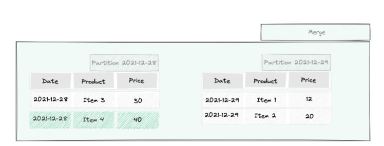
  • Merge incoming data with existing data by keeping the newest version of each record.

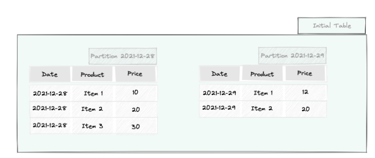
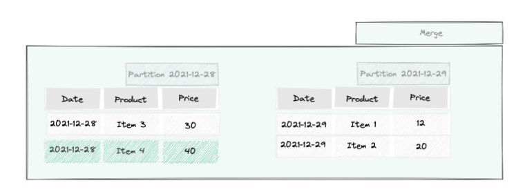
For performance reasons, when having huge amount of data, tables are usually split into multiple partitions. BigQuery supports range partitioning which are uncommon and date/time partitioning which is the most widely used type of partitioning. The diagram below shows our initial table partitioned by the date field.

Initial data

Let's assume we receive the following data that we need to ingest into the table:

Incoming data

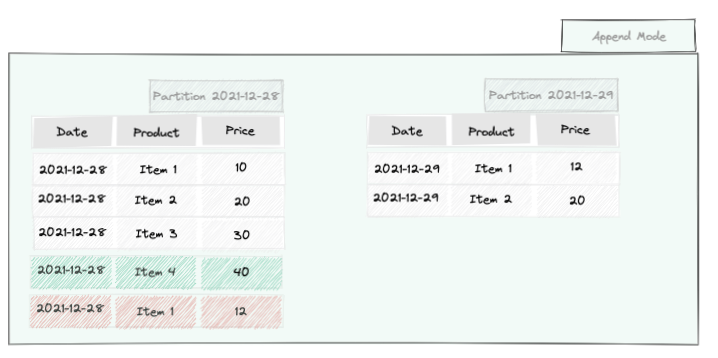
The strategies above will produce respectively the results below:

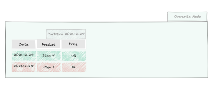
The table ends up with the 2 incoming records. All existing partitions are deleted.

Overwrite data

There is no good or bad strategy, the use of one of the strategies above depends on the use case. Some use case examples for each of the strategies are:

  • Overwrite mode may be useful when you receive every day the list of all product names.
  • Append mode may be useful when you receive daily sales.
  • Dynamic Partition Overwrite mode may be useful when you ingested the first time a partition, and you need to ingest it again with a different set of data and thus alter only that partition.
  • Merge mode may be useful when you receive product updates every day and that you need to keep only the last version of each product.

Spark How-to

Apache Spark SQL connector for Google BigQuery makes BigQuery a first class citizen as a source and sink for Spark jobs.

Append and Overwrite modes in Spark

BigQuery is supported by Spark as a source and sink through the Spark BigQuery connector

Spark comes out of the box with the ability to append or overwrite existing data using a predefined save mode:


val incomingDF = ... // Incoming data loaded with the correct schema
val bqTable = "project-id.dataset.table"
val saveMode = SaveMode.Overwrite // or SaveMode.Append fot he appending data
incomingDF.write
.mode(saveMode)
.partitionBy("date")
.format("com.google.cloud.spark.bigquery")
.option("table", bqTable)
.save()

Dynamic Partition Overwrite mode in Spark

To activate dynamic partitioning, you need to set the configuration below before saving the data using the exact same code above:

spark.conf.set("spark.sql.sources.partitionOverwriteMode","DYNAMIC")

Unfortunately, the BigQuery Spark connector does not support this feature (at the time of writing). We need to manually delete the partitions we want to overwrite first and then append the incoming data.

Assuming the table is partitioned by the field date and the incoming data loaded in the incomingDF dataframe, the code below will remove existing partitions that need to be overwritten.

Delete partitions that need to be updated
val incomingDF = ... // Incoming data loaded with the correct schema
incomingDF
.select(date_format(col("date"), "yyyyMMdd").cast("string"))
.distinct()
.collect()
.map(_.getString(0))
.foreach { partition =>
bigQueryClient.deleteTable(TableId.of(datasetName, s"$table\$$partition"));
}
tip

To drop a table partition using the Google Cloud bq command line tool, you may use the following syntax:

bq rm -t 'project-id.dataset.table$YYYYMMDD'

We now need to append the incomingDF to mimic the dynamic partition overwrite feature:

Append incoming partitions
val incomingDF = ... // Incoming data loaded with the correct schema
val bqTable = "project-id.dataset.table"
val saveMode = SaveMode.Append
incomingDF.write
.mode(saveMode)
.partitionBy("date")
.format("com.google.cloud.spark.bigquery")
.option("table", bqTable)
.save()
caution

The issue with this approach is that if the program crashes during the "appending" of the incoming data, partitions will have been deleted and data would be lost. However, you can still ingest the same file again in case of failure and the end result will be the same.

Dynamic Partition Merge in Spark

When you need to keep the last version of the record for each product, both BigQuery and Databricks (the company behind Spark in case you lived on the moon the last ten years) support the merge SQL statement:

Merge records using SQL statement
MERGE INTO target_table
USING incoming_table
ON target_table.product = incoming_table.product
WHEN NOT MATCHED
THEN INSERT *
WHEN MATCHED AND incoming_table.date > target_table.date THEN
UPDATE SET *
/*
WHEN MATCHED AND incoming_table.timestamp <= target_table.timestamp THEN
SKIP
*/

Unfortunately the MERGE statement is not supported by Apache Spark. It is only supported by Databricks, its commercial version.

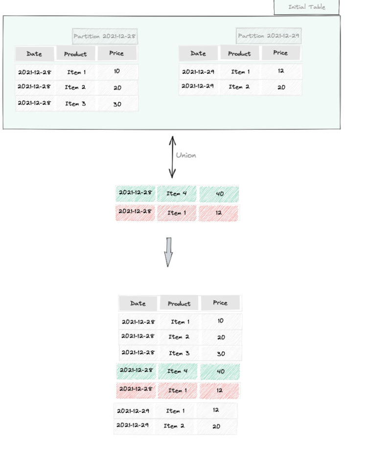
To do a merge using the Spark BigQuery connector, we need to do it by following the steps below:

Step 1: Create a dataframe with all the rows

val allRowsDF =
incomingDF
.unionByName(existingDF)

Step 1

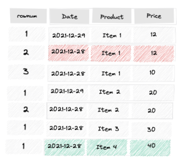
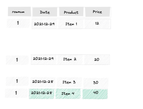
Step 2: group by product and order each product occurrence by date descending

val orderingWindow =
Window
.partitionBy("product")
.orderBy(col("date").desc, col("product")))

val orderedDF =
allRowsDF
.withColumn("rownum", row_number.over(orderingWindow))

Step 2

In the step 2 above, each product is ordered by date with the most recent one first (descending order). We identify it by the rownum column.

Step 3: Keep the most recent product

val toKeepDF =
orderedDF
.where(col("rownum") === 1)
.drop("rownum")

Step 3

Step 4: Overwrite existing partitions with the data we want to keep


val bqTable = "project-id.dataset.table"
val saveMode = SaveMode.Overwrite
toKeepDF.write
.mode(saveMode)
.partitionBy("date")
.format("com.google.cloud.spark.bigquery")
.option("table", bqTable)
.save()

Step 4

Starlake How-to

Starlake is a declarative Ingestion Framework based on YAML description files.
The 4 ingestion strategies described above are supported through the settings below:

Schema Definition File
     name: "mydb"
directory: "..."
+ metadata:
schemas:
- name: "mytable"
pattern: "data-.*.csv"
metadata:
writeStrategy:
type: "OVERWRITE"
attributes:
- name: "date"
type: "date"
rename: "id"
- name: "product"
type: "string"
- name: "price"
type: "decimal"

See again manual Spark overwrite